Central Limit Theorem

In this blog, let’s focus on skew normal distribution.

The probability density function with location ξ , scale ω , and slant α

Mean: ${\displaystyle \xi +\omega \delta {\sqrt {\frac {2}{\pi }}}}$ where ${\displaystyle \delta ={\frac {\alpha }{\sqrt {1+\alpha ^{2}}}}}$

Variance: ${\displaystyle \omega ^{2}\left(1-{\frac {2\delta ^{2}}{\pi }}\right)}$

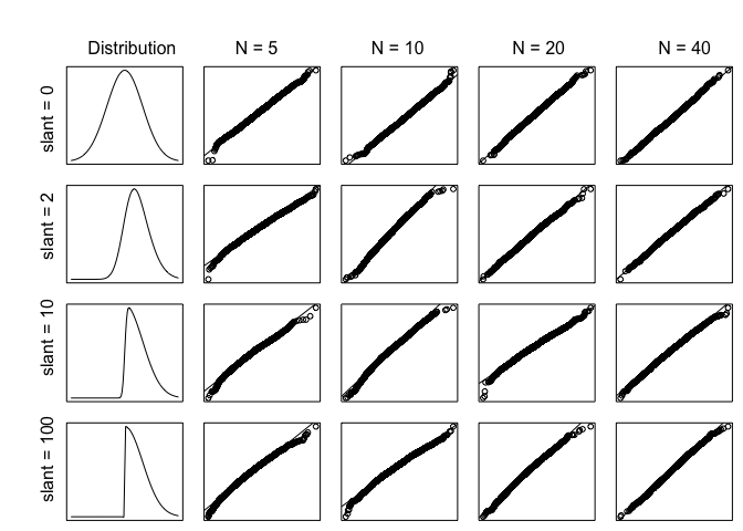
In this simulation, set location and scale to 0 and 1. Slant will be set to 0, 2, 10, 100 and sample size will be set to 5, 10, 20, and 40.

Let’s generate a sampling distribution of 5000 draws from both the CLT approximation and the simulation approximation.

The output of each combination of factors will be a QQ-plot with CLT approximation on the y axis and simulation approximation on the x aixs.

CLT shortcut

If $Z_{\alpha}$ is a quantile of the standard normal, then $Z_{\alpha}\frac{v}{\sqrt{N}} + m$ is an approximate quantile of the sampling distribution of $\bar{X}_N$ when the conditions of CLT are met.

For the purposes of this simulation, let’s treat the mean and variance as known values and use the actual population parameters and the population mean and variance instead of sample estimates.

R <-5000
location <- 0
scale <- 1

#Parameters that change
generate_qqplot <- function(N,slant){

delta <- slant / (sqrt(1 + slant ^ 2))
pop_mean <- location + scale * delta * sqrt(2 / pi)
pop_sd <- sqrt(scale ^ 2 * (1 - (2 * delta ^ 2) / pi))

Z <- rnorm(R)
#CLT approximation
sample_dist_clt <- Z*(pop_sd/sqrt(N))+pop_mean

#Simulation approximation
random.skew <- array(rsn(R*N,xi=location,omega=scale,alpha=slant),dim=c(R,N))

sample_dist_sim <-apply(random.skew,1,mean)

#QQ plot
qqplot(sample_dist_sim,sample_dist_clt,axes = FALSE, frame.plot=TRUE, ann = FALSE)
abline(0,1)
  
}

par(mfrow=c(4,5),mai=c(0.1,0.1,0.1,0.1), oma = c(0, 4, 4, 0))
#Parameters that change
slant <- c(0,2,10,100)
N <- c(5,10,20,40)
x <- seq(-3,3,by=0.05)

#call the function for different slant and N
for (s in slant){
  plot(dsn(x, xi = location,omega = scale, alpha = s), type = "l",axes = FALSE, frame.plot=TRUE)
  for (n in N){
    generate_qqplot(n,s)
  }
}

#add text
mtext('slant = 100        slant = 10        slant = 2        slant = 0'
      , side = 2, outer = TRUE)
mtext('Distribution            N = 5                   N = 10                  N = 20                   N = 40'
      , side = 3, outer = TRUE)

The table of figures above are the results. We could see that as the slant increases, there will be more deviation in tails. As the sample size increases, the plotted points will fall along the line y=x more approximately.