Coverage Probability

21 Oct 2019

Reading time ~3 minutes

Introduction

Coverage probability is an important operating characteristic of methods for constructing interval estimates, particularly confidence intervals. In this blog, we will focus on 95% confidence interval of median from maximum likelihood estimation and then calculate the proportion of the time that the interval contains the true value of median, which is coverage probability.

Generate Data

First, let’s generate a single sample from a standard normal distribution of size N=201 use rnorm function.

N <- 201
pop.mean = 0
pop.sd = 1
true.parameters <- c(N,mean = pop.mean, sd = pop.sd)

generate_data <- function(parameters){
  data=rnorm(parameters[1],parameters[2],parameters[3])
}

Use MLE to Estimate the Distribution**

For the normal model, the MLE solution is $\hat{\mu} = \bar{X};\ \ \widehat{\sigma^2} = \frac{N-1}{N}s^2\approx s^2$

Thus, we could use MLE to estimate the distribution of the single sample we generated before.

est.mle <- function(data){
  mle.mean <- mean(data)
  mle.sd <- sd(data)
  return(c(length(data),mle.mean,mle.sd))
}

true.parameters %>% generate_data %>% est.mle

## [1] 201.0000000  -0.1013798   1.1379364

We could see that the the mean and standard deviation for the generated sample is about 0 and 1, but with slight difference.

Get Confidence Interval

Then let’s construct a confidence interval for the median

confidence interval

After using mle to estimate the mean and standard deviation of sample with size 201, we could use these parameters to generate sample and compute the median for this sample. Repeat this process 5000 times and we will get 5000 sample median.

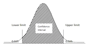
Let’s define the 95% confidence interval of the median to be the middle 95% of sampling distribution of the median.

The lower confidence limit for median is 0.025 quantile and the upper confidence limit for median is 0.975 quantile.

boot.meds.ci <- function(parameters){
  R <- 5000
  sample.meds <- NA
  for (i in 1:R){
    sample.meds[i] <- parameters %>% generate_data()%>% median
  }
  quantile(sample.meds,c(0.025,0.975))
}

Capture Median

The median for standard normal distribution is 0. A confidence interval will capture median if the lower confidence limit is less than zero and the upper confidence limit is greater than zero. Then let’s set a function to test whether the confidence interval captured the true median or not. The function will return 1 if the confidence interval captured the true median and return 0 if the confidence interval didn’t capture the true median.

capture_median <- function(ci){
  1*(ci[1]<0 & 0<ci[2])
}

Coverage Probability

The coverage probability is the proportion of the time that the interval contains the true value of interest.

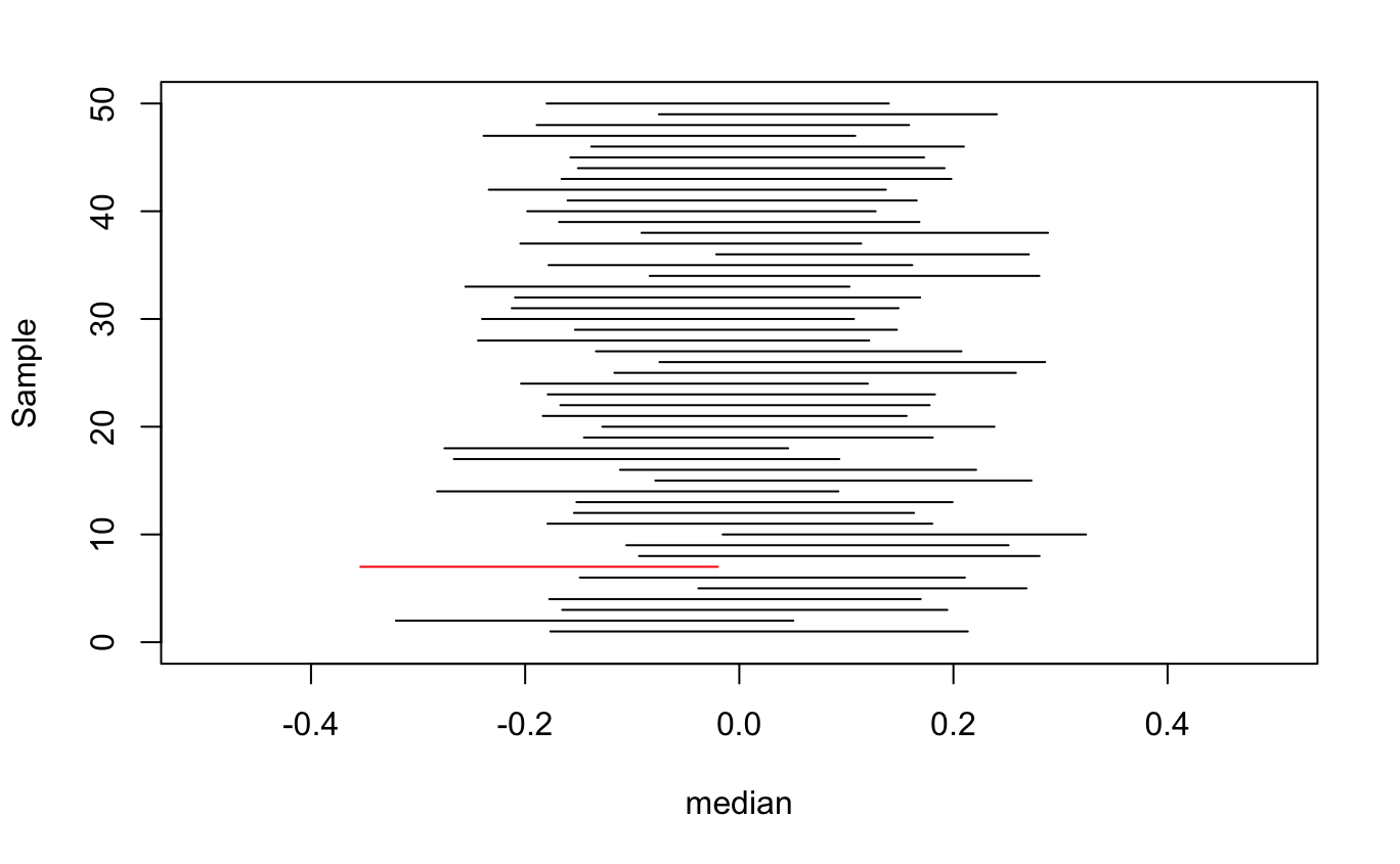
The figure above shows the 95% confidence interval calculated for 50 samples. Intervals in black capture the population parameter of interest; intervals in red do not. Thus, in this case the coverage probability is 49/50.

Estimate the Coverage Probability for Median

Now let’s take 95% confidence interval calculated for 5000 samples and compute the coverage probability as the proportion of samples for which the confidence interval captured the true value of median.

Repeat the function we generated before: generate_data %>% est.mle %>% boot.meds.ci **%>% **capture_median 5000 times and then compute the mean of captures as coverage probability.

M <- 5000
captures <- rep(NA, M) 
for(i in 1:M){
  captures[i] <- true.parameters %>% generate_data %>% est.mle %>% boot.meds.ci %>% capture_median

} 
capture_prob <- mean(captures)

capture_prob

## [1] 0.9848

The coverage probability for 5000 simulation is 0.9848. Idealy, a 95% confidence interval will capture the population parameter of interest in 95% of samples and our simulations perform a little bit better than 95%.