Home field advantage
The home field advantage is the edge which a team may have when playing a game at its home stadium. For example, it is the edge the Braves may have over the Yankees when the head-to-head match-up is in Atlanta. It is the advantage the Yankees may have when the head-to-head match-up is in New York.
The term is widely used in best-of-seven playoff formats as being given to the team that is scheduled to play one more game at home than their opponent if all necessary games are played.
Suppose best-of-seven series follow a “2-3-2” format, the sequence of game locations is {NYC, NYC, ATL, ATL, ATL, NYC, NYC}
In a 2-3-2 series, the first two games are played at the home venue of a team with the better regular-season record, the next three games (including the fifth, if necessary) are played at the home of the team with the worse regular-season record, and the final two games (if necessary) are played at the home of the team with the better regular-season record
Assumption
| Probability | Definition |
|---|---|
| PB | the probability that the Braves win a single head-to-head match-up with the Yankees, under the assumption that home field advantage doesn’t exist |
| PBH | the probability that the Braves win a single head-to-head match-up with the Yankees as the home team (H for home) |
| PBA | the probability that the Braves win a single head-to-head match-up with the away team (A for away) |
| Game location | No advantage | Advantage |
|---|---|---|
| ATL | PB | PBH = PB * 1.1 |
| NYC | PB | PBA = 1 − (1 − PB) * 1.1 |
Statistical Method
Let’s assume PB = 0.55
| Game location | No advantage | Advantage |
|---|---|---|
| ATL | PB = 0.55 | PBH = PB * 1.1 = 0.605 |
| NYC | PB = 0.55 | PBA = 1 − (1 − PB) * 1.1 = 0.505 |
With Home Filed Advantage
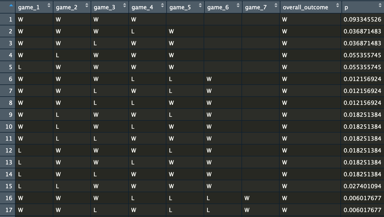
There are 70 all-possible-world-series-outcomes, 35 for overall win and 35 for overall lose.

For example, in this case, the probability that the Braves win the world series when the sequence of game locations is {NYC, NYC, ATL, ATL, ATL, NYC, NYC} will be PBA * PBA * PBH * PBH = 0.0933
We calculate the probability of each possible outcome, then sum up the probability for wins as analytical probability that the Braves win the world series.


require(dplyr)
require(data.table)
# Get all possible outcomes
apo <- fread("all-possible-world-series-outcomes.csv")

# Home field indicator
hfi <- c(0,0,1,1,1,0,0) #{NYC, NYC, ATL, ATL, ATL, NYC, NYC}

# P_B
pb <- 0.55
advantage_multiplier <- 1.1 # Set = 1.1 for advantage
pbh <- 0.55*advantage_multiplier
pba <- 1 - (1 - 0.55)*advantage_multiplier

# Calculate the probability of each possible outcome
apo[, p := NA_real_] # Initialize new column in apo to store prob
for(i in 1:nrow(apo)){
  prob_game <- rep(1, 7)
  for(j in 1:7){
    p_win <- ifelse(hfi[j], pbh, pba)
    prob_game[j] <- case_when(
        apo[i,j,with=FALSE] == "W" ~ p_win
      , apo[i,j,with=FALSE] == "L" ~ 1 - p_win
      , TRUE ~ 1
    )
  }
  apo[i, p := prod(prob_game)] # Data.table syntax
}

# Sanity check: does sum(p) == 1?
#apo[, sum(p)] # This is data.table notation

# Probability of overall World Series outcomes
apo[, sum(p), by=overall_outcome]
##    overall_outcome       V1
## 1:               W 0.604221
## 2:               L 0.395779
overall_win=apo[overall_outcome=="W"]
pro_with_adv=sum(overall_win$p)
pro_with_adv
## [1] 0.604221
Analytically, the probability that the Braves win the world series with home field advantage when PB=0.55 is 0.604221
Without Home Field Advantage
For best-of-7 match-up, the Braves could win the series in 4,5,6 or 7 games
For a team to win the series in game N, they must have won exactly 3 of the first N-1 games and won the last game
| win the series in game N | situation | probability |
|---|---|---|
| 4 | 3 wins in 3 & win last game | dnbinom(0,4,0.55) |
| 5 | 3 wins in 4 & win last game | dnbinom(1,4,0.55) |
| 6 | 3 wins in 5 & win last game | dnbinom(2,4,0.55) |
| 7 | 3 wins in 6 & win last game | dnbinom(3,4,0.55) |
pro_without_adv=pnbinom(3,4,0.55)
pro_without_adv
## [1] 0.6082878
Analytically, the probability that the Braves win the world series without home field advantage when PB=0.55 is 0.6082878.
Difference in Probabilities
pro_with_adv-pro_without_adv
## [1] -0.004066825
The difference in probabilities is -0.004066825. Since Yankees could play one more game in their home field than Braves, Yankees have the overall home field advantage. Thus, the difference in probabilities with and without home field advantage for Braves is negative.
Simulation Method
With Home Field Advantage
Now let’s compute the probability in a simulation way. For each simulation, we randomly generate the results for 7 games, either win or lose. If braves win equal to or more than four games, the overall outcome will be win. Otherwise,the overall outcome will be lose.
Run 100,000 times simulation, the probability that the Braves win the world series is the ratio that Braves win among the 100,0000 simulations.
# Home field indicator
hfi <- c(0, 0, 1, 1, 1, 0, 0) #{ATL, ATL, NYC, NYC, NYC, ATL, ATL}
advantage_multiplier <- 1.1 # Set = 1 for no advantage
pbh <- 0.55 * advantage_multiplier
pba <- 1 - (1 - 0.55) * advantage_multiplier

#simulation for one game
win_lose <- rep(NA, 100000)
for (j in 1:100000) {
result <- rep(NA, 7)
for (i in 1:7) {
p_win <- ifelse(hfi[i], pbh, pba)
result[i] = rbinom(1, 1, p_win)
if (sum(result, na.rm = TRUE) == 4) {
win_lose[j] = 'W'
break
}
else if (length(result[which(result == 0)]) == 4) {
win_lose[j] = "L"
break
}
else
next
}
}
pro_simu_with_adv=mean(win_lose == 'W')
pro_simu_with_adv
## [1] 0.60584
Without Home Field Advantage
If home filed advantage does not exist, we set the advantage multiplier to be 1 for no advantage.
Same as before, let’s run 100,000 times simulation, the probability that the Braves win the world series is the ratio that Braves win among the 100,0000 simulations.
# Home field indicator
hfi <- c(0, 0, 1, 1, 1, 0, 0) #{ATL, ATL, NYC, NYC, NYC, ATL, ATL}
advantage_multiplier <- 1 # Set = 1 for no advantage
pbh <- 0.55 * advantage_multiplier
pba <- 1 - (1 - 0.55) * advantage_multiplier

#simulation for one game
win_lose <- rep(NA, 100000)
for (j in 1:100000) {
result <- rep(NA, 7)
for (i in 1:7) {
p_win <- ifelse(hfi[i], pbh, pba)
result[i] = rbinom(1, 1, p_win)
if (sum(result, na.rm = TRUE) == 4) {
win_lose[j] = 'W'
break
}
else if (length(result[which(result == 0)]) == 4) {
win_lose[j] = "L"
break
}
else
next
}
}
pro_simu_without_adv=mean(win_lose == 'W')
pro_simu_without_adv
## [1] 0.60753
Absolute Error and Relative Error for simulation
Simulation generates approximate answers; there is some degree of error in a quantity estimated by Monte Carlo simulation. What’s the absolute error and relative error in our simulation?
Definition:
absolute error = |p̂ − p|
relative error = |p̂ − p|/p
Thus, the p̂ would be the probability we calculated in simulation and p would be the analytical probability we computed in first section.
Here are the results
Absolute Error (with home field advantage)
abs_error_with_adv=abs(pro_simu_with_adv-pro_with_adv)
abs_error_with_adv
## [1] 0.001619028
Relative Error (with home field advantage)
rel_error_with_adv=abs(pro_simu_with_adv-pro_with_adv)/pro_with_adv
rel_error_with_adv
## [1] 0.00267953
Absolute Error (without home field advantage)
abs_error_without_adv=abs(pro_simu_without_adv-pro_without_adv)
abs_error_without_adv
## [1] 0.0007577969
Relative Error (without home field advantage)
rel_error_without_adv=abs(pro_simu_without_adv-pro_without_adv)/pro_without_adv
rel_error_without_adv
## [1] 0.001245787
Does the difference in probabilities (with vs without home field advantage) depend on PB
Our previous assumption is PB=0.55, now let’s set a series of PB, from 0.5 to 0.9, then see how the difference in probabilities would change over PB
| Game location | No advantage | Advantage |
|---|---|---|
| ATL | PB | PBH = PB * 1.1 |
| NYC | PB | PBA = 1 − (1 − PB) * 1.1 |
Set PB from 0.5 to 0.9, with break 0.001. Then compute the analytical probability that the Braves win the world series for each PB
p_with_adv=rep(NA,400)
p_without_adv=rep(NA,400)
# Get all possible outcomes
for (k in 1:400){
apo <- fread("all-possible-world-series-outcomes.csv")

# Home field indicator
hfi <- c(0,0,1,1,1,0,0) #{NYC, NYC, ATL, ATL, ATL, NYC, NYC}

# P_B
pb <- 0.5+0.001*k
advantage_multiplier <- 1.1 # Set = 1.1 for advantage
pbh <- pb*advantage_multiplier
pba <- 1 - (1 - pb)*advantage_multiplier

# Calculate the probability of each possible outcome
apo[, p := NA_real_] # Initialize new column in apo to store prob
for(i in 1:nrow(apo)){
  prob_game <- rep(1, 7)
  for(j in 1:7){
    p_win <- ifelse(hfi[j], pbh, pba)
    prob_game[j] <- case_when(
        apo[i,j,with=FALSE] == "W" ~ p_win
      , apo[i,j,with=FALSE] == "L" ~ 1 - p_win
      , TRUE ~ 1
    )
  }
  apo[i, p := prod(prob_game)] # Data.table syntax
}


# Sanity check: does sum(p) == 1?
#apo[, sum(p)] # This is data.table notation

# Probability of overall World Series outcomes
apo[, sum(p), by=overall_outcome]
overall_win=apo[overall_outcome=="W"]
p_with_adv[k]=sum(overall_win$p)
p_without_adv[k]=pnbinom(3,4,0.5+0.001*k)
}
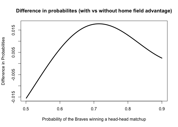
Here is the plot for difference in probabilites (with vs without home field advantage) and PB
plot(seq(0.501,0.9,0.001),p_with_adv-p_without_adv,type='l',lwd=3,xlab='Probability of the Braves winning a head-head matchup',ylab='Difference in Probabilities',main="Difference in probabilites (with vs without home field advantage)")

We could see that the difference in probabilities would increase and then decrease over a series of PB, from 0.5 to 0.9. When PB is greater than 0.6, the difference in probabilities start to be positive, indicating that Braves have a bigger chance to win the world series with home field advantage than it does without home filed advantage.
Does the difference in probabilites (with vs without home field advantage) depend on the advantage factor?
Our previous assumption is advantage factor = 1.1, that results in a 10% increase for the home team.
Now let’s set a series of advantage factor, from 1 to 1.8, with break 0.01. Then see how the difference in probabilities would change over advantage factor.
| Game location | No advantage | Advantage |
|---|---|---|
| ATL | PB = 0.55 | PBH = 0.55 * AdvantageFactor |
| NYC | PB = 0.55 | PBA = 1 − (1 − 0.55) * AdvantageFactor |
p_with_adv=rep(NA,80)
p_without_adv=rep(NA,80)
# Get all possible outcomes
for (k in 1:80){
apo <- fread("all-possible-world-series-outcomes.csv")

# Home field indicator
hfi <- c(0,0,1,1,1,0,0) #{NYC, NYC, ATL, ATL, ATL, NYC, NYC}

# P_B
pb <- 0.55
advantage_multiplier <- 1+0.01*k # Set = 1.1 for advantage
pbh <- pb*advantage_multiplier
pba <- 1 - (1 - pb)*advantage_multiplier

# Calculate the probability of each possible outcome
apo[, p := NA_real_] # Initialize new column in apo to store prob
for(i in 1:nrow(apo)){
  prob_game <- rep(1, 7)
  for(j in 1:7){
    p_win <- ifelse(hfi[j], pbh, pba)
    prob_game[j] <- case_when(
        apo[i,j,with=FALSE] == "W" ~ p_win
      , apo[i,j,with=FALSE] == "L" ~ 1 - p_win
      , TRUE ~ 1
    )
  }
  apo[i, p := prod(prob_game)] # Data.table syntax
}


# Sanity check: does sum(p) == 1?
#apo[, sum(p)] # This is data.table notation

# Probability of overall World Series outcomes
apo[, sum(p), by=overall_outcome]
overall_win=apo[overall_outcome=="W"]
p_with_adv[k]=sum(overall_win$p)
p_without_adv[k]=pnbinom(3,4,0.55)
}
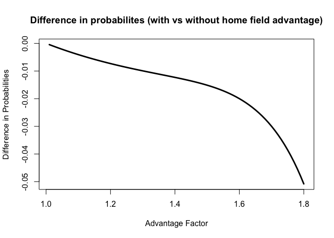
Here is the plot for difference in probabilites (with vs without home field advantage) and Advantage Factor
plot(seq(1.01,1.8,0.01),p_with_adv-p_without_adv,type='l',lwd=3,xlab='Advantage Factor',ylab='Difference in Probabilities',main="Difference in probabilites (with vs without home field advantage)")

It is clear that the difference in probabilities would decrease over a series of advantage factor, from 1 to 1.8. However, we should notice that the difference is negative. Thus, when we take absolute value, the absolute value for difference in probabilities actually increases as advantage factor increases.
As advantage factor increases, probability to win in Atlanta PBH = 0.55 * advantage factor will increases, and probability to win in New York PBA = 1 − (1 − 0.55) * advantage factor will decrease. Since Yankees can play one more game at their home field, the probability that the Braves win world series with home filed advantage will decrease as advantage factor increases.