Motivation
A common research objective is to demonstrate that two measurements are highly correlated.
For example,
A measurement: reflect the severity of disease but is difficult or costly to collect.
B measurement: easier to collect and potentially related to measurement A.
Thus, if there is strong association between A and B, a cost effective strategy for diagnosis may be to collect measurement B instead of A.
Power Calculation
Power is the probability that the study will end in success when the true underlying correlation is, in fact, greater that 0.8
Recall that, a type II error is made if we fail to reject the null hypothesis when in fact the null hypothesis is false
Thus, power = 1 - Type II error (β)
In this blog, we will estimate power for different combinations of sample size and the true population correlation
Let the sample size be 25, 50, 75, and 100. Let the population correlation range from 0.8 to 0.95.
| Correlation | A | B |
|---|---|---|
| A | 1 | rho |
| B | rho | 1 |
First, we generate a vector of random values from an N-dimensional multivariate normal distribution given some mean vector and covariance matrix
For instance, if we set N = 10, the generated data would be like this
##              [,1]        [,2]
##  [1,] -1.98630078 -1.88018692
##  [2,] -1.08606909 -2.96877559
##  [3,]  0.15626669 -0.95789487
##  [4,] -0.16431225  0.08264868
##  [5,]  1.65431451  0.65172155
##  [6,]  0.48730551  0.85109515
##  [7,]  0.43559321  0.71010025
##  [8,]  0.01193761  0.26670785
##  [9,] -1.95107450 -1.92285104
## [10,] -0.80914405 -1.09479418
Take 5000 simulations, power is the proportion of the time that the true underlying correlation between A and B is greater than 0.8
Our hypothesis is:
H0 : p<=0.8
H1 : p>0.8
generate_plot <- function(N){
power=rep(NA)
N
null_correlation <- 0.8
R <- 5000
mu <- c(0,0)

for (j in 1:16){
  sigma <- array(c(1,0.79+0.01*j,0.79+0.01*j,1), c(2,2))
  detect <- rep(NA, R)
  for(i in 1:R){
  data <- rmvnorm(N, mean = mu, sigma = sigma)
  results <- cor.test(x = data[,1], y = data[,2], alternative = "greater")
  detect[i] <- results$conf.int[1] > null_correlation
  }
  power[j] <- mean(detect)
}
lines(seq(0.8,0.95,0.01),power,type='l',col=N,pch=16,lwd=3)
text(0.87,power[8],paste0("N=",N),pos=2,cex=0.7,col=N)

}
The plot of power for different combinations of sample size and the true population correlation is shown below
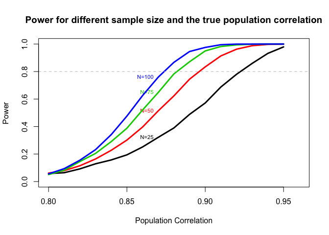
As true population correlation increases, the power(the probability that the study will end in success) will increase.
As sample size increases, the power will will increase.
Thus, if we want two measurements to be highly correlated, we could collect measurements on more individuals or choose measurements with larger true population correlation.