Simulation generates approximate answers and there is some degree of error in a quantity estimated by Monte Carlo simulation. In this blog, we are going to investigate the relationship between then number of replicates and simulation error.
Definition
p̂:the probability estimated from simulation
p: the true underlying probability
absolute error = |p̂ − p|
relative error = |p̂ − p|/p
14 X 5 Factorial Experiment Simulation
replicate number: (22, 23, …, 215)
probability: (0.01, 0.05, 0.10, 0.25, 0.50)
We first generate matrix for each combination of replicate number and probability, then perform a 14 X 5 factorial experiment simulation
#generate matrix for each combination of replicate number and probability
abs_error=matrix(NA,14,5)
rel_error=matrix(NA,14,5)
p=c(0.01, 0.05, 0.10, 0.25, 0.50)
#perform a 14 X 5 factorial experiment simulation
for (i in 1:14){
  for (j in 1:5){
    p_hat=rbinom(10000,2^(i+1),p[j])/(2^(i+1))
    abs_error[i,j]=mean(abs(p_hat-p[j]))
    rel_error[i,j]=mean(abs(p_hat-p[j])/p[j])
  }
}
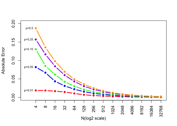
Figure: Absolute Error
x_axis=c("4","8","16","32","64","128","256","512","1024","2048","4096","8192","16384","32768")
prob=c("0.01","0.05","0.10","0.25","0.5")
prob_label=paste0("p=",prob)
plot(as.vector(abs_error[,1]),xaxt='n',type="b",col="red",lwd=3,pch=20,xlim=c(0,14),ylim=c(0,0.2),xlab="N(log2 scale)",ylab="Absolute Error")
axis(1,at=1:14,labels=x_axis,las=2)
lines(as.vector(abs_error[,2]),type="b",col="blue",lwd=3,pch=20)
lines(as.vector(abs_error[,3]),type="b",col="green",lwd=3,pch=20)
lines(as.vector(abs_error[,4]),type="b",col="purple",lwd=3,pch=20)
lines(as.vector(abs_error[,5]),type="b",col="orange",lwd=3,pch=20)
text(1,abs_error[1,],prob_label,pos=2,cex=0.7)

The absolute error declines a lot when N is between 4 and 64 and stays very samll after N exceeds 8192.
The degree of absolute error gets smaller as the number of simulation replicates increases.
For p=0.01, its original absolute error’s value is the smallest among five probabilities.
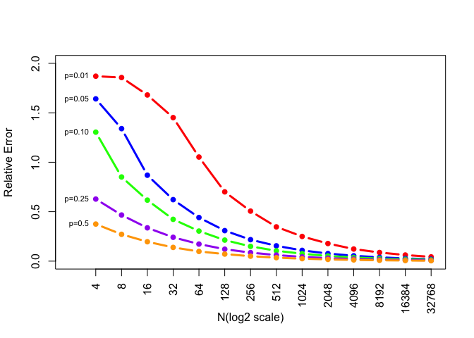
Figure: Relative Error
x_axis=c("4","8","16","32","64","128","256","512","1024","2048","4096","8192","16384","32768")
prob=c("0.01","0.05","0.10","0.25","0.5")
prob_label=paste0("p=",prob)
plot(as.vector(rel_error[,1]),xaxt='n',type="b",col="red",lwd=3,pch=20,xlim=c(0,14),ylim=c(0,2),xlab="N(log2 scale)",ylab="Relative Error")
axis(1,at=1:14,labels=x_axis,las=2)
lines(as.vector(rel_error[,2]),type="b",col="blue",lwd=3,pch=20)
lines(as.vector(rel_error[,3]),type="b",col="green",lwd=3,pch=20)
lines(as.vector(rel_error[,4]),type="b",col="purple",lwd=3,pch=20)
lines(as.vector(rel_error[,5]),type="b",col="orange",lwd=3,pch=20)
text(1,rel_error[1,],prob_label,pos=2,cex=0.7)

The reletive error declines a lot when N is between 4 and 64 and stays very samll after N exceeds 8192.
The degree of relative error gets smaller as the number of simulation replicates increases.
For p=0.5, its original relative error’s value is the smallest among five probabilities.
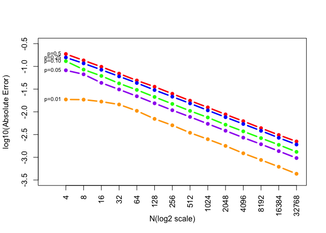
Figure: Absolute Error (with the y-axis is on the log10 scale)
Now let’s take log10 for absolute error and generate a new plot
x_axis=c("4","8","16","32","64","128","256","512","1024","2048","4096","8192","16384","32768")
prob=c("0.01","0.05","0.10","0.25","0.5")
prob_label=paste0("p=",prob)
plot(log10(as.vector(abs_error[,5])),xaxt='n',type="b",col="red",lwd=3,pch=20,xlim=c(0,14),ylim=c(-3.5,-0.5),xlab="N(log2 scale)",ylab="log10(Absolute Error)")
axis(1,at=1:14,labels=x_axis,las=2)
lines(log10(as.vector(abs_error[,4])),type="b",col="blue",lwd=3,pch=20)
lines(log10(as.vector(abs_error[,3])),type="b",col="green",lwd=3,pch=20)
lines(log10(as.vector(abs_error[,2])),type="b",col="purple",lwd=3,pch=20)
lines(log10(as.vector(abs_error[,1])),type="b",col="orange",lwd=3,pch=20)
text(1,log10(abs_error[1,]),prob_label,pos=2,cex=0.7)

We can see that it seems to be a linear relationship between log10(absolute error) and N(log2 scale).
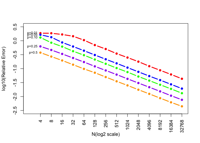
Figure: Relative Error (with the y-axis is on the log10 scale)
Let’s also take log10 for relative error and generate a new plot
x_axis=c("4","8","16","32","64","128","256","512","1024","2048","4096","8192","16384","32768")
prob=c("0.01","0.05","0.10","0.25","0.5")
prob_label=paste0("p=",prob)
plot(log10(as.vector(rel_error[,1])),xaxt='n',type="b",col="red",lwd=3,pch=20,xlim=c(0,14),ylim=c(-2.5,0.5),xlab="N(log2 scale)",ylab="log10(Relative Error)")
axis(1,at=1:14,labels=x_axis,las=2)
lines(log10(as.vector(rel_error[,2])),type="b",col="blue",lwd=3,pch=20)
lines(log10(as.vector(rel_error[,3])),type="b",col="green",lwd=3,pch=20)
lines(log10(as.vector(rel_error[,4])),type="b",col="purple",lwd=3,pch=20)
lines(log10(as.vector(rel_error[,5])),type="b",col="orange",lwd=3,pch=20)
text(1,log10(rel_error[1,]),prob_label,pos=2,cex=0.7)

We can see that it also seems to be a linear relationship between log10(relative error) and N(log2 scale).
Conclusion
From the four graphs, we can see that our intuition is right. That is, the degree of error gets smaller as the number of simulation replicates increases.
And for log 10 scale, the figures of the absolute error and relative error shows that there is a linear relationship between absolute error/relative error(log10 scale) and N(log2 sacale).
For p=0.01, its original absolute error’s value is the smallest among five probabilities.
For p=0.5, its original relative error’s value is the smallest among five probabilities.